Week 1 | Elec3030

1.0 Test and Measurement

OBJECTIVES

GOALS

The objective of this lab is to familiarize the student with lab equipment that will be regularly used in ELEC 3030.

Chapter 1 Goals

Become familiar with lab test equipment
- AFG1062 Arbitrary Function Generator
- Tektronix MDO 3032 Oscilloscope
- Tenma DC power supply
- Omega HHM90 digital multimeter (DMM)
Generate and measure sine waves
Become familiar with amplitude modulation
Generate and measure an AM signal

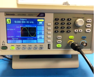
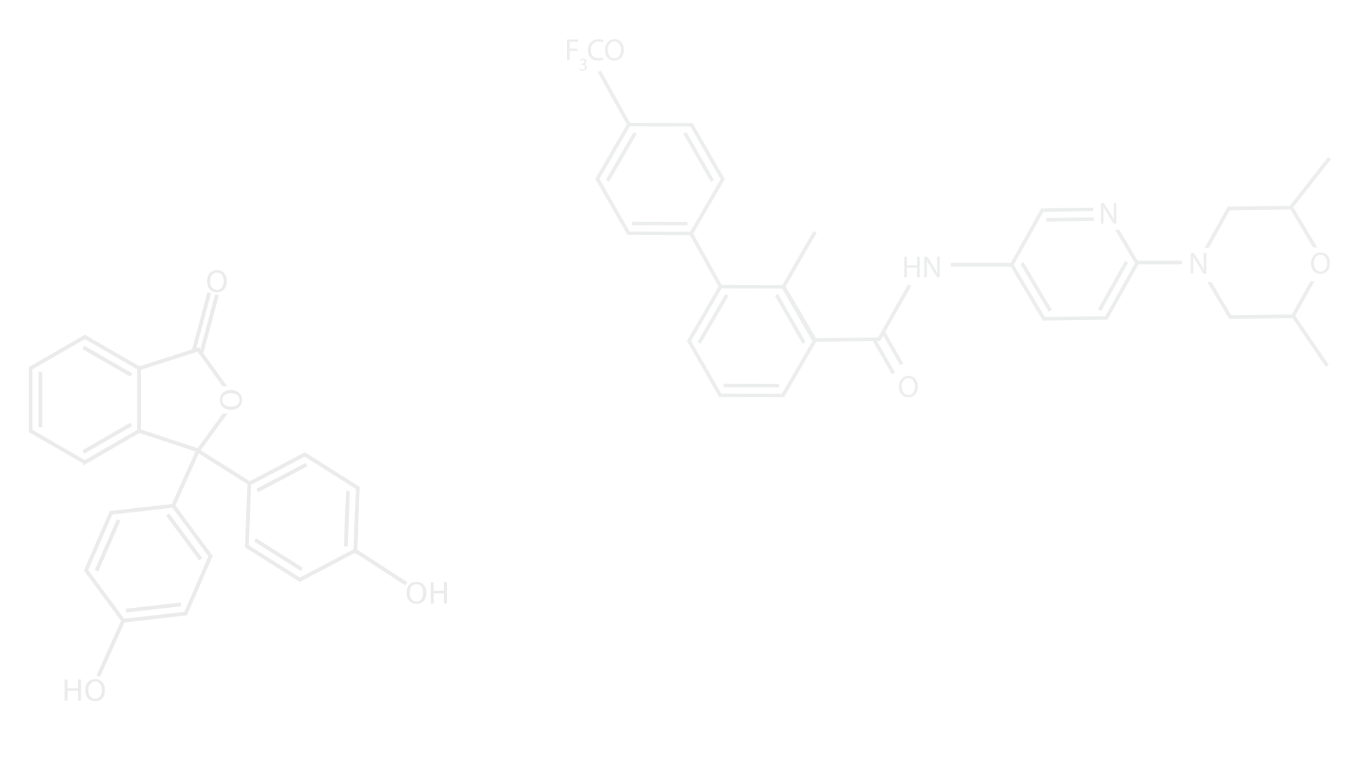
Figure 1: AFG1062 Arbitrary Function Generator

Figure 2: Tektronix MDO 3032 Oscilloscope

2 Vpp, 10 kHz sine wave displayed on Oscilloscope

Figure 3: 2 Vpp Sine Wave at 10 kHz

Figure 4: 2 Vpp Sine Wave with Cursors

Figure 5: Amplitude Modulated Signal at 10 kHz

Figure 6: Spectrum of AM waveform with 50% modulation

Figure 7: Spectrum of AM waveform with 100% modulation

Table 1: Spectrum information at 50% modulation

Table 2: Spectrum information at 100% modulation

Figure 8: Amplitude Modulated Signal at 50 kHz with FFT

Figure 9: Spectrum of FFT Waveform with 50% modulation

Figure 10: Spectrum of FFT Waveform with 100% modulation

Table 3: Spectrum information at 50% modulation

Table 4: Spectrum information at 100% modulation

1.1 Simple Sine Waves

For the first section of the lab, I will be using the AFG 1062 Function Generator (FGEN), shown in Figure 1, to produce a 1 V amplitude 10 kHz sine wave and view the output on the MDO 3032 oscilloscope (O-scope), shown in Figure 2. When configuring the FGEN, I set the "High" amplitude or maximum voltage, to 1 V and the "Low" amplitude to -1 V. This is equivalent to a peak-to-peak voltage of 2 V. There is no DC Offset voltage and the frequency of the signal is set to 10 kHz. Using a BNC-to-BNC cable, I plugged one end into the Channel 1 output port on the FGEN and the other end into the Channel 1 port on the O-scope. With the 'Trigger Level' knob and 'Acquire' button, the scope was adjusted until the clear sine wave in Figure 3 was displayed. The 'Trigger' knob helped steady the signal while the 'Acquire' button averaged the data to sharpen it.

Once the sine wave was displayed, I took advantage of the 'Cursors' button at the top of the O-scope to measure the peak-to-peak voltage of the signal. By pressing the 'Cursors' button and positioning each vertical cursor at each peak of the signal, the "delta" displayed should read approximately 2 V to represent the change from the high amplitude to the low amplitude. I also made sure to display the frequency at the bottom of the display by using the 'Measure' button to select 'Add Measurement' and include the frequency. The results are then displayed in Figure 4.

It is also beneficial to verify that the desired timescale is set appropriately when operating the O-scope. Since signal frequencies are represented with Hertz and the period of a signal is the inverse of the frequency, I can use their relationship to adjust the timescale close to the period. For example, if given a 10 kHz signal, the timescale should be set to 100 us.

Next, I disconnected the frequency generator to view the sine wave on the Omega Digital Multimeter (DMM). With the DMM set to read 20 V AC, the output of the FGEN was probed and recorded at 1.63 V. This value was expected because the DMM measures the peak-to-peak value and divides it by the square root of two to get the Root-mean-square (RMS) value.

1.2 Amplitude Modulation

I then focused on analyzing an intelligence signal to observe amplitude modulation. An intelligence signal is an audio signal of voice or music that is carried along a carrier wave to modulate the amplitude of the carrier. In this lab experiment, a small carrier frequency is used for better visualization of an AM signal. With that being said, a signal with a 1 kHz intelligence frequency and a 1 MHz carrier frequency should have a time scale closer to 1 ms instead of 1 us to see the intelligence signal.

While keeping the generator frequency high at 10 kHz, an amplitude modulated signal was created by first engaging an internal modulation within the FGEN using a 1 kHz signal as the carrier frequency. The modulation on the generator was set to 50% and the time scale to 400 us. Adjusting the voltage and amplitude scales in addition to moving the trigger allowed me to analyze the steady signal shown in Figure 5.

After that, the student then created another amplitude modulated signal using the spectrum analyzer on the O-scope. First, the cable from the O-scope's output was disconnected. Then, the carrier frequency was increased to 1230 kHz and the amplitude was set to 100 mVpp. The DC offset, intelligence signal, and modulation depth all remained 0 V, 1 kHz, and 50% respectively. Once the BNC-to-BNC is connected to the Radio Frequency (RF) input of the O-scope, the student configured the center frequency to 1.23 MHz, the span to 50 kHz, and the reference label to 0 dBm. The resolution bandwidth was set to 200 Hz and the spectrum of the AM signal is displayed in Figure 6. The same steps were then repeated for the same amplitude modulated signal with a 100% modulation depth and displayed in Figure 7.

Using the markers, the student recorded the readings for both signals into Table 1 and Table 2.

1.3 AM Signal Frequency Spectrum (FFT Method)

Finally, I will analyze the AM signal using the O-scope's fast Fourier transform (FFT) function because it separates the signal into the frequencies that make it up. For this portion of the lab, the FGEN is set to output a 50 kHz sine wave with a 100 mV peak-to-peak value and the internal modulation is set to 1 kHz with a depth of 50%. Using the Math button on the O-scope and ensuring that the time base reads 400 us, I analyzed the signal shown in Figure 8 and then selected the FFT operation to display the signal shown in Figure 9. I quickly noticed that the results in Figure 9 are similar to the ones analyzed in Figure 6 as they should be. The same steps were again repeated for the same amplitude modulated signal with a 100% modulation depth and displayed in Figure 10. The frequencies, dB levels, and voltage amplitudes were finally recorded into Tables 3 and 4.

Reflective Writing

This lab served as an introduction to equipment that will be heavily used throughout the remainder of the semester. Previously, I had experience with using the built-in function generator and oscilloscope within the National Instruments ELVIS board and analyzing signals with a LABVIEW program created by the professor. In this lab, I was able to use both on a larger scale. I quickly learned that the process of analyzing signals in this case involves a lot more technical application, but I was able to quickly adapt.